Tidy Tuesday 2023-12-05

This Tidy Tuesday was about life expectancy from Our World in Data and I decided to participate for the first time. The data and instructions can be found here: TidyTuesday 2023-12-05.

After looking at the summary, I quickly decided upon looking at the differences in life expectancy between women and men and whether they changed over time. Time was restricted to 1950 to 2020 to only look at current erra and benefit from classification of countries based on income.

Code

df <- tuesdata$life_expectancy_female_male %>%
  filter(Entity %in% c("High-income countries", "Upper-middle-income countries", "Lower-middle-income countries", "Least developed countries", "Low-income countries")) %>%
  mutate(
    le_fm = LifeExpectancyDiffFM,
    Entity = factor(Entity, levels = c("High-income countries", "Upper-middle-income countries", "Lower-middle-income countries", "Least developed countries", "Low-income countries"))
  )

# General life expectancy
p1 <- filter(tuesdata$life_expectancy, Year >= 1950) %>%
  ggplot(aes(x = Year, y = LifeExpectancy)) +
  geom_line(aes(group = Entity), col = "grey80", alpha = 0.7, linewidth = 0.5) +
  geom_smooth(se = F, col = "#527853", linewidth = 2) +
  theme_minimal() +
  ylab("Life expectancy") +
  xlab("")

# Life expectancy difference between Female and Male
p2 <- filter(tuesdata$life_expectancy_female_male, Year >= 1950) %>%
  ggplot(aes(x = Year, y = LifeExpectancyDiffFM)) +
  geom_line(aes(group = Entity), col = "grey80", alpha = 0.7, linewidth = 0.5) +
  geom_smooth(se = F, col = "#527853", linewidth = 2) +
  ylab("Females vs Males") +
  xlab("") +
  labs(title = "Life expectancy difference") +
  scale_y_continuous(limits = c(0, 10)) +
  theme_minimal()

# By country type

p3 <- filter(df, Year >= 1950) %>%
  ggplot(aes(x = Year, y = le_fm, col = Entity)) +
  geom_line(aes(group = Entity), col = "grey80", alpha = 0.7, linewidth = 0.5) +
  geom_smooth(se = F, linewidth = 2) +
  facet_grid(cols = vars(Entity)) +
  theme_classic() +
  theme(
    strip.background = element_blank(),
    legend.position = "none"
  ) +
  ylab("Females vs Males") +
  scale_colour_brewer(palette = "Oranges")


p1 / p2 / p3

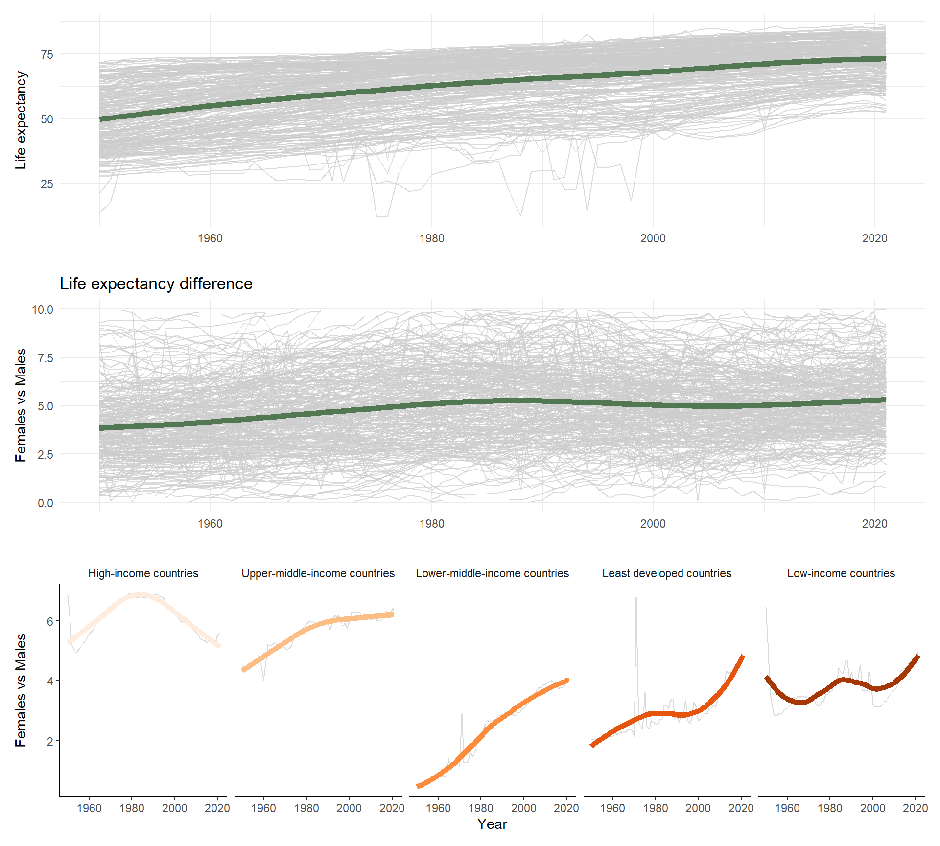
At the same time that life expectancy is increasing, the gap between women and men is also becoming larger. This is especially true for middle and low income countries. In high income countries, the gap is now reducing. Still, women life expectancy is 4 years higher compared to men.

Code

# Some code used to explore the data.
map(tuesdata, summary)

map(tuesdata, naniar::vis_miss)

tuesdata$life_expectancy_female_male %>%
  group_by(Entity) %>%
  filter(Year >= 1950) %>%
  summarise(mean_se(LifeExpectancyDiffFM)) %>%
  arrange(ymin)

tuesdata$life_expectancy_female_male %>%
  filter(Entity == "United Kingdom") %>%
  View()

tuesdata$life_expectancy_female_male$Entity %>%
  unique() %>%
  str_subset("countr")

model <- tuesdata$life_expectancy_female_male %>%
  filter(Year >= 1870) %>%
  lm(le_fm ~ Year + Entity, data = .)

model %>%
  broom::tidy() %>%
  arrange(estimate) %>%
  View()